Method

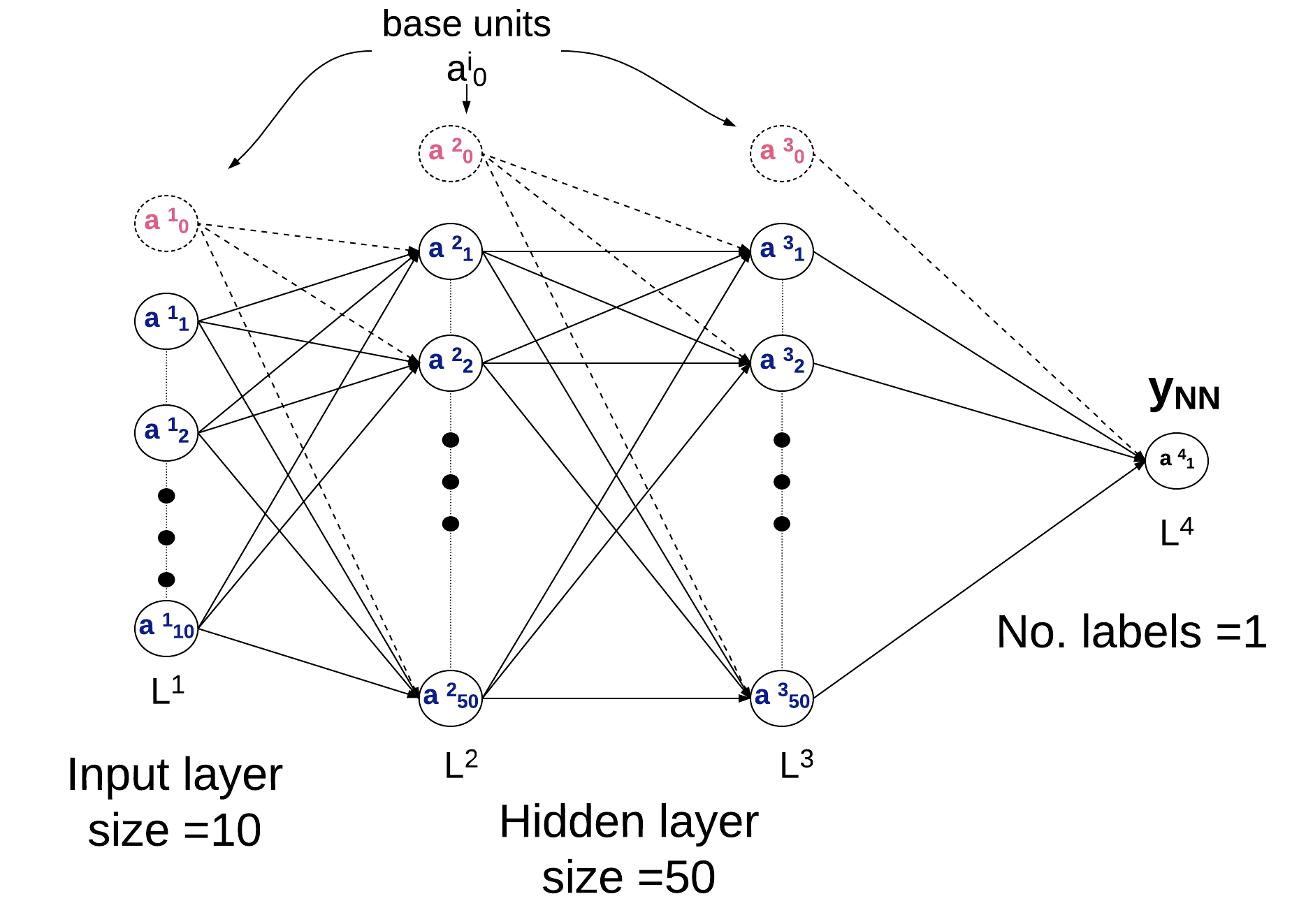
The neural network is set up as shown in the figure below.

The network is trained on the training set. The procedure is as follows

1. Decide on the input parameters for the data (x), the number of hidden layers and the number of nodes in each hidden layer.

2. Initialise the weights of the network. These will be randomly generated numbers, our starting point. As the network runs these weights become optimised as the neural network learns which information is important to correctly guess the catagory of the object. The weights connect each node in the previous layer to each node in the present layer, thus the weights are a matrix with size ((N _{layer_i} +1) x N _{layer_j} ) where j = i+1. NB there is an extra node added in layer_i which is the zero node or base unit.

3. Using the initial weights, compute how well the network predicts the true outcome. For layers 1 to 4 (i.e input, 2 x hiddenlayers and output) we compute the following (the superscript denotes the layer number):

   $$\color{black} \begin{align*} & a^{(1)} = \mathbf{x}, \quad \textrm{add}\quad a_0^{(1)}\\ & z^{(2)} = \Theta^{(1)}a^{(1)}, \quad a^{(2)} = \frac{1}{(1 + \exp{-z^{(2)}})}, \quad \textrm{add}\quad a_0^{(2)} \\ & z^{(3)} = \Theta^{(2)}a^{(2)}, \quad a^{(3)} = \frac{1}{(1 + \exp{-z^{(3)}})}, \quad \textrm{add}\quad a_0^{(3)} \\ & z^{(4)} = \Theta^{(3)}a^{(3)}\\ & y_{NN} = a^{(4)} = \frac{1}{(1 + \exp{-z^{(4)}})}\\ \end{align*}$$
   • Different functions can be used here but we use the cost function to descibe how close our model is to predicting the correct classification. It is defined as
   $$\color{black} J(\mathbf{\Theta}) = -\frac{1}{m} \sum_{i=1}^{m} y^i \log y_{NN}(\mathbf{\Theta})^i + (1-y^i)\log(1-y_{NN} (\mathbf{\Theta})^i) + \frac{\lambda}{m}\sum_{i=1}^{L-1}\mathrm{tr}(\mathbf{\Theta}^T\mathbf{\Theta})$$
   • where m is the number of data points in the sample, L are the total number of layers and
   $$\color{black} \mathrm{tr}(A^T A) = \sum_{i=1}^n \sum_{j=1}^m a_{i,j}^2$$

4. To reduce the cost function and train the network we then work backwards (back propagation) to compute the gradient of the cost function which we can feed in our our optimiser inorder for it to search for the Theta parameters that return minimum cost and therefore best model the training data.

   • We compute a delta for layers L down to 2.
   $$\color{black} \delta^{(L)} = y_{NN} - y$$ $$\color{black} \delta^{(L-i)} = \mathbf{\Theta}^{(L-i) \mathbf{T}} \delta^{(L-i+1)} a^{(L-i)}(1-a^{(L-i)})$$
   • The gradient at each layer (l) and each unit (j) in that layer is
   $$\color{black} \frac{\partial J}{\partial \Theta_j} = \sum_{i=1}^{m} \frac{1}{m} a_j^{(l)}\delta^{(l+1)} + \sum_{i=1, j\neq 0}^{m}\lambda \Theta_j^{(l)}.$$

5. With the cost function and gradient of cost function algorithm we can now take advantage of built-in optimisation routines in python. I have used the scipy.optimize.fmin_cg function.

6. Now the neural network is set up we can test that the gradients are being computed correctly by running a small sample through our gradient computation routine and comparing the outcome with that from a simple finite difference routine.

7. If that looks good the next step is computing the best regularisation parameter Lambda, and the number of nodes required in the hidden layers using the cross-validation data set.

8. We chose the values of Lambda and the number of hidden layer nodes as those that give the lowest cost-function/highest accuracy on our cross-validation data set.

9. Now we can train the network using these values and see how well it performs on the test data set as a function of the number of iterations required by the optimisation function.

UPDATE: I found that it was more efficient to use the sklearn.neural_network.MLPClassifier. The new code has been added to the repo, and I will be updating the results section.